14  Combined Loads

NoteLearning Objectives

• Determine total normal stress resulting from combinations of normal forces, bending moments, and pressure
• Determine total shear stress when transverse loads in one or both transverse directions are combined with torsional loads
• Determine the general stress state when any combination of the above is applied and use those results to determine principal stresses and principal stress planes

This chapter uses all the previously discussed concepts to determine the total normal stress and the total shear stress for a body subjected to various types of loading simultaneously. Axial forces (Chapter 5), bending moments (Chapter 9), and pressure (Chapter 13) may be applied in various combinations to give total normal stress. Transverse loads (Chapter 10) in multiple directions and torsion (Chapter 6) can combine to give total shear stress.

Understanding which loads lead to which types of stresses and in which directions requires having a good grasp of coordinate axes. In particular being able to distinguish between the longitudinal axis and the cross-sectional axes is important. This can change from body to body as different coordinate axes are used, but it can also change within an individual body according to changes in geometry. Section 14.1 reviews how to distinguish between the coordinate axes as well as defines generic terms that will allow us to express equations in a more generalized manner.

Section 14.2 reviews and expands on the various sources of normal stress. These normal stresses will be reframed in terms of the general axes discussed in @sect-14.1 so as to clarify which other normal stresses they may combine with. Section 14.2.1 revisits bending stress to express the unsymmetric bending stress equation in terms of general cross-sectional axes. Section 14.2.3 considers eccentric loading, which is a specific instance of combined normal stress in which normal forces result in bending.

Section 14.3 focuses on combining the various sources of shear stress to determine the total shear stress. To expand on the concepts discussed and used in Chapter 6 and Chapter 10, here we perform calculations based on both possible transverse loading directions as well as torsion. As in Section 14.2, this is accomplished using a general set of coordinate axes.

Section 14.4 further expands the above cases to situations in which all combinations of loading are possible and the general stress state is determined.

Note that determining internal reactions for the general problems presented in this chapter requires the use of 3D equilibrium equations, particularly for determining bending moments and torsion. You may thus find it helpful to review Section 1.4 to understand these calculations.

14.1 Coordinate Axes and Directions

Click to expand

To generalize the discussion for any set of coordinate axes, we will use generic terms for the various directions, as shown in Figure 14.1. The vertical axis of the cross-section will be referred to as the V axis, the horizontal axis of the cross-section will be referred to as the H axis, and the longitudinal (axial) direction will be referred to as the L axis.

The longitudinal direction, synonymous with axial direction, is the direction perpendicular to a cross-section that is cut at a point of interest on a body. The cross-sectional axes are the axes drawn on the cross-section based on viewing the cross-section down the longitudinal axis.

Figure 14.1: To maintain generality, we use V to denote the vertical axis of the cross-section, H to denote the horizontal axis of the cross-section, and L to denote the longitudinal axis of the body based on the cross-section of interest.

These directions could change from point to point depending on the location of the point of interest and the geometry of the body. For example, consider the structure in Figure 14.2 with the x-, y-, z-axes oriented at the origin as shown. To examine point P on the structure, we make a vertical cut at point P. The direction normal to the cut surface is the x direction, so the x-axis is the longitudinal axis. When viewing the cut surface looking down the x-axis, you see the y-axis and z-axis on the cross-section, so those are the cross-sectional axes. In this view, the y-axis appears to be the vertical (V) axis of the cross-section and the z-axis is horizontal (H).

In contrast, for point Q we must make a horizontal cut to examine that point. The normal direction to the cut is then the vertical, or y-axis, and the cross-sectional axes as viewed looking down the y-axis are the x-axis and z-axis. In this view, the x-axis would appear to be the horizontal axis of the cross-section and the z-axis would appear to the vertical axis of the cross-section.

Depending on your perspective, you may switch the cross-sectional axes you consider to be horizontal versus vertical. Ultimately this will not matter as long as you correctly distinguish between the longitudinal and cross-sectional directions.

Figure 14.2: The longitudinal (L), horizontal (H), and vertical (V) axes depend on how the axes are arranged globally for the structure as well as on the specific location of the point in question.

In the following sections we will express equations in terms of these generic directions so that they will apply to any orientation of coordinate axes.

14.2 Combined Normal Stress

Click to expand

Previous chapters considered individual sources of longitudinal normal stress: axial loads (Chapter 5), bending loads (Chapter 9), and pressure loads (Chapter 13). With all three of these forms of loading present we can express the generalized equation for total longitudinal stress as

\[ \sigma_L =\frac{\sum F_L}{A}+\sigma_{bending}+\frac{p r}{2 t}\text{ ,} \]

where
𝜎_L = Total normal stress in the longitudinal direction [Pa, psi]
F_L = Force in the longitudinal direction [N, lb]
A = Cross-sectional area [m², in.²]
𝜎_bending = Bending stress (discussed in more detail below) [Pa, psi]
p = Internal pressure [Pa, psi]
r = Inner radius of pipe or pressure vessel [m, in.]
t = Wall thickness of pipe or pressure vessel [m, in.]

If there is pressure loading in addition to the contribution to the longitudinal normal stress indicated above, there will also be normal stress in the cross-sectional directions equal to the hoop stress.

\[\sigma_V=\sigma_H=\sigma_{hoop}=\frac{pr} {t}\]

Of course, for problems without pressure, the pressure terms would be excluded.

Of the three types of longitudinal normal stress, bending stress tends to be the most complex to understand in terms of calculation inputs and signs, especially with varying coordinate axes directions. Section 14.2.1 revisits the concept of bending stress to discuss how to generalize the Chapter 9 equations to any orientation of body with any arrangement of coordinate axes.

14.2.1 Generalized Bending Stress Equation

Section 9.3 derived an equation for bending stress in the x direction based on bending around the cross-sectional axes y and z. That equation is

\[ \sigma_x=-\frac{M_z y}{I_z}+\frac{M_y z}{I_y} \]

The minus sign in front of the M_z term and the plus sign in front of the M_y term are part of the derived equation. When the correct signs for M_z, M_y, y, and z are inserted, the correct sign of the stress is obtained (positive for tensile and negative for compressive). Note that Chapter 9 considered no other cross-sectional axes so that focus on the general concept of bending stress could be more easily maintained.

When the cross-sectional axes are not y and z, we apply the same general form of the above bending stress equation. However, for a different set of axes, we not only need to change the bending moment and second moment of area axes in the equation but also need to reconsider the signs in front of each term. In any given bending load situation the bending moments are the moments around the centroidal axes of the cross-section (V and H) and the resulting normal stress is in the longitudinal direction (L).

Given this information, we can then reframe the bending stress equation in a generalized form.

\[ \boxed{{\sigma_{(bending)}= \pm\left|\frac{M_V\ d_H}{I_V}\right| \pm\left|\frac{M_H\ d_V}{I_H}\right|}}\text{ ,} \tag{14.1}\]

where
𝜎(_bending) = Bending stress in the longitudinal direction [Pa, psi]
M_V = Bending moment around the vertical axis of the cross-section [N⸱m, lb⸱in.]
M_H = Bending moment around the horizontal axis of the cross-section [N⸱m, lb⸱in.]
d_H = Horizontal distance between the point of interest on the cross-section and the V-axis [m, in.]
d_V = Vertical distance between the point of interest on the cross-section and the H-axis [m, in.]
I_V = Second moment of area about the vertical axis of the cross-section [m⁴, in.⁴]
I_H = Second moment of area about the horizontal axis of the cross-section [m⁴, in.⁴]

Figure 14.3 illustrates the distances d_H and d_V for the case where the stress at the example point P on the cross-section is being calculated.

The absolute values used for the bending stress terms with the ± in front indicate that we will calculate the magnitude of each bending stress term and then assess the signs of the terms independently. We assess the signs by visualizing the bending direction or by using visualization tools, described below. Recall that compressive stresses are considered negative and tensile stresses are positive.

Also helpful to note is that M_H does not affect the normal stress of points directly on the H-axis and M_V does not affect the normal stress of points directly on the V-axis. This is evident from the fact that d_H = 0 for a point on the V-axis and d_V = 0 for a point on the H-axis.

Figure 14.3: The distances d_H and d_V that would go in Equation 14.1 when calculating the bending stress for the example point P on the cross-section

14.2.2 Assessing Bending Stress Signs for Generalized Bending Stress Equation

The sign on each of the two bending stress terms in Equation 14.1 is determined by inspection of the bending direction. Section 9.1, showed that a bending moment around the horizontal axis causes the normal stress to vary along the vertical axis of the cross-section. Section 9.3 showed that a bending moment around the vertical axis causes normal stress to vary across the cross-section’s horizontal axis. Which side is in tension versus compression in each case depends on the direction (clockwise versus counterclockwise) of the bending moment as well as the location of the point on the body.

If we can visualize the expected bending direction due to loading, we can assess whether a point will be on the “inside” of the bend (compression) or on the “outside” of the bend (tension). For example, in Figure 14.4 the rightward horizontal force results in bending around the V-axis of the cross-section. The direction of the bending is such that all points to the right of the V-axis on the cross-section are on the inside of the bend (compression) and all points to the left of the V-axis on the cross-section are on the outside of the bend (tension).

In Figure 14.5, the force in the V direction results in a bending moment around the H-axis. The direction of the bending is such that all points above the H-axis on the cross-section are on the inside of the bend (compression) and all points below the H-axis on the cross-section are on the outside of the bend (tension).

Figure 14.4: Bending around the V-axis

Figure 14.5: Bending around the H-axis

If visualization is difficult, use the following tool (refer to Figure 14.6):

1. Draw the cross-section as viewed from the free end or cut end toward the origin. For example, in the case of the columns in Figure 14.4 and Figure 14.5, we would draw the top-down view of the cross-section.
2. Draw the bending moment arrows around the V-axis and H-axis on the sketch of the cross-section. Exaggerate the arrows so they are drawn all the way across.
   • Make sure to draw the bending moment arrows such that they cross over (or in front of) the bending axis (as opposed to under or behind).
3. The side the arrowhead points to is the compressive side, and the side the tail of the arrow is on is the tensile side.

This approach is demonstrated for the bending stress calculation in Example 14.1.

Figure 14.6: Bending moments drawn around vertical and horizontal axes shown with exaggerated moment arrows to assess tension versus compression.

TipExample 14.1

Example 14.1  

The internal bending moments on a 32 mm diameter solid steel rod are found to be M_x = 376 kN·mm (clockwise) and M_z = 204 kN·mm (counterclockwise) as shown.

Determine the bending stress at points P and Q.

TipSolution

1. Normally, the first step is to draw the free body diagram (FBD) of the cut section to find the internal bending moments. In this case, for simplicity, the internal moments are already given.

2. Write the general bending stress equation and eliminate unnecessary terms.

\[ \sigma_L= \pm\left|\frac{M_H\ d_V}{I_H}\right| \pm\left|\frac{M_V\ d_H}{I_V}\right| \]

Looking at the cross-section, we can see that the cross-sectional vertical axis is the z-axis and the cross-sectional horizontal axis is the x-axis. The longitudinal axis is the y-axis.

\[ \sigma_y= \pm\left|\frac{(M_z)\ (d_x)}{I_z}\right| \pm\left|\frac{(M_x)\ (d_z)}{I_x}\right| \]

Evaluating point P:

Because P is on the centroidal z-axis, d_x = 0, and the general bending stress equation reduces to

\[ \sigma_y= \pm\left|\frac{(M_x)\ (d_z)}{I_x}\right| \]

3. Assess the sign.

With the clockwise bending moment around the x-axis, the beam can be visualized as bending backward such that point P will be on the inside of the bend, or in compression. An approximation of the resulting shape is sketched here as it would appear from the side view (looking down the x-axis).

Alternatively, draw the cross-section with the exaggerated moment arrow clockwise around the x-axis. Since the arrowhead would be pointed toward P, the point is in compression.

4. Calculate the values.

|M_x| = given = (376 kN·mm)(1,000 N/kN) = 376,000 N·mm

d_z = radius = 16 mm

I_x =\(\frac{\pi}{64}d^4=\frac{\pi}{64}(32mm)^4=51.47\times10^3mm^4\)

\[ \begin{aligned} \sigma_{y_P}&=-\frac{376,000{~N}\cdot{mm}\ (16mm)}{51.47 \times 10^{3}{~mm}^4}\\[10pt] &=-117{~N/mm^2}\\[10pt] &=-117\ MPa \end{aligned} \]

Evaluating Point Q:

Because point Q is on the centroidal x-axis, d_z = 0, so the general bending stress equation reduces to

\[ \sigma_{y_Q}=\pm\left|\frac{(M_z)\ (d_x)}{I_z}\right| \]

3. Assess the sign.

With the counterclockwise bending moment around the z-axis, the beam can be visualized as bending into somewhat of a backward “C” shape as viewed from the front (down the z-axis). Point Q would be on the outside of the bend, or in tension.

Alternatively, draw the cross-section with the exaggerated moment arrow counterclockwise around the z-axis. Since Q is at the tail side, the point is in tension.

4. Calculate the values.

|M_z| = given = (204 kN·mm)(1,000 N/kN) = 204,000 N·mm

d_x = radius = 16 mm

For the circular cross-section, I_z = I_x = 51.47 x 10³ mm⁴.

\[ \begin{aligned} \sigma_{y_Q}&=\frac{204,000{~N}\cdot{mm}*(16{~mm})}{51.47 \times 10^{3}{~mm}^4}\\[10pt] &=63.4\ N/mm^2\\[10pt] &=63.4{~MPa} \end{aligned} \]

Answer:

σ_yP = 116.9 MPa (Compression)

σ_yQ = 63.4 MPa (Tension)

14.2.3 Eccentric Loading

When the line of action of an axial load doesn’t pass through the centroid of a cross-section, it results in both a normal reaction force and a bending moment. For example, consider the traffic light and corresponding FBD shown in Figure 14.7.

Figure 14.7: The vertical pole is subject to direct axial stress and bending stress.

The vertical support pole is subjected to normal forces from the weights of the traffic lights (the weight of the horizontal poles, cameras, etc. are assumed to be negligible for this example). Also, bending moments around both cross-sectional axes (x and z) result from the weights not being directly centered on the support pole.

The total normal stress in the longitudinal direction, σ_L, at any given point on the pole would be given by

\[ \sigma_L =\frac{\sum F_L}{A}+\sigma_{bending} \]

In terms of the general axes discussed in Section 14.1, and substituting in Equation 14.1 for the bending stress, we have

\[ \boxed{{\sigma_L= \pm\left|\frac{F_L}{A}\right| \pm\left|\frac{M_V\ d_H}{I_V}\right| \pm\left|\frac{M_H\ d_V}{I_H}\right|}}\text{ ,} \tag{14.2}\]

where
𝜎_𝐿 = Bending stress in the longitudinal direction [Pa, psi]
F_L = Internal normal force in the longitudinal direction [N, lb]
A = Cross-sectional area [m², in.²]
M_V = Bending moment around the vertical axis of the cross-section [N⸱m, lb⸱in.]
M_H = Bending moment around the horizontal axis of the cross-section [N⸱m, lb⸱in.]
d_H = Horizontal distance between the point of interest on the cross-section and the V-axis [m, in.]
d_V = Vertical distance between the point of interest on the cross-section and the H-axis [m, in.]
I_V = Second moment of area about the vertical axis of the cross-section [m⁴, in.⁴]
I_H = Second moment of area about the horizontal axis of the cross-section [m⁴, in.⁴]

The sign for the first term is positive if the F_L is tensile (directed away from the cross-section) and negative if F_Lis compressive (pointed toward the cross-section).

Example 14.2 and Example 14.3 demonstrate the calculation of normal stress in eccentric loading problems.

Example 14.4 demonstrates a loading that includes pressure as part of the loading combination and drawing the resulting stress element.

TipExample 14.2

Example 14.2  

The structure is fixed to the ground and subjected to the 75 lb and 50 lb vertical forces shown.

Determine the total normal stress at points P and Q on the cross-section located at A-A. Assume the 40 in. horizontal section at the top remains rigid.

TipSolution

1. Draw the FBD of the structure cut at A-A and write the equilibrium equations to find the internal reactions.

Below is the FBD for the section of the structure above the cut. Using the section above the cut allows us to avoid needing to calculate the reactions at the fixed support.

In this case reaction forces R_x and R_z are 0 by inspection (note that no forces are applied in those directions).

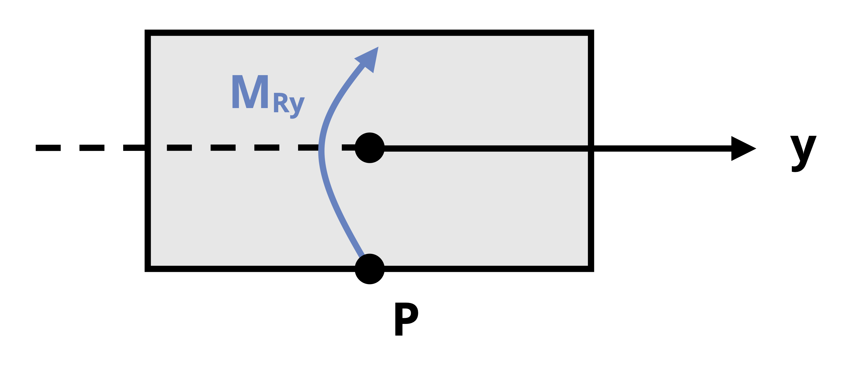
Similarly, reaction moments M_Rx and M_Ry are 0 by inspection: All the forces act only in the y direction, so M_Ry = 0. All the forces pass through the x-axis, so M_Rx = 0.

Calculate R_y and M_Rz.

\[\begin{aligned}\sum F_y=R_y-75{~lb}-50{~lb}=0 \quad\rightarrow\quad R_y=125{~lb}\end{aligned}\] \[\begin{aligned}\sum\ M_z &=\sum\pm(Fy*x)+\sum \pm\ (Fx*y)+M_{Rz}=0\\[10pt] &=(75{~lb}*15{~in.})-(50{~lb}*25{~in.})+M_{Rz}=0 \quad\rightarrow\quad M_ {Rz}=125{~lb}\cdot{in.}\end{aligned}\]

Remember when calculating reaction moments to calculate moments about the centroidal axes of the cross-section no matter where on the cross-section the point of interest lies.

2. Write the generalized normal stress equation and eliminate unnecessary terms.

\[ \sigma_L= \pm\left|\frac{F_L}{A}\right| \pm\left|\frac{M_V\ d_H}{I_V}\right| \pm\left|\frac{M_H\ d_V}{I_H}\right| \]

Here the longitudinal axis is the y-axis. The vertical axis of the cross-section is the z-axis, and the horizontal axis is the x-axis. With M_Rx = 0, we have

\[ \sigma_y= \pm\left|\frac{R_y}{A}\right| \pm\left|\frac{M_{Rz}\ d_x}{I_z}\right| \]

3. Assess signs.

According to the equilibrium equations applied in step 2, the following is true:

R_y points toward the cut section, so it is compressive (negative). In addition, the force affects all points on the cross-section in the same way, so the R_y/A term is negative for both points P and Q.

M_Rz is counterclockwise for the section of the body above the cut at A-A.

However, correctly visualizing bending direction tends to be easier if we consider the direction of the bending moment for the section of the body attached to the fixed support. In this case that is the section below the cut. Because the reactions on either side of the cut act in opposing directions (equal/opposite reactions), the section attached to the fixed support is subjected to a clockwise bending moment.

The opposing reactions at the cut are shown here, as well as a sketch of the body bending clockwise around the z-axis and a top down view of the cross-section with the moment arrow going clockwise around the z-axis.

Given the above, note that point P will be in tension (outside of bend) from the bending stress and point Q will be compression (inside of bend).

4. Calculate the stress.

In addition to R_y and M_Rz, the following are required:

A = (6in.)(8in.) = 48 in.²

d_x for point P = x distance between P and the z-axis = 2 in.

d_x for point Q = x distance between Q and the z-axis = 4 in.

\[ I_z = \frac{1}{12}bh^3=\frac{1}{12}(6{~in.})(8{~in.})^3 = 256{~in.^4} \]

Evaluate point P.

\[ \sigma_{yP}=-\left|\frac{125{~lb}}{48{~in.^2}}\right|+\left|\frac{(125{~lb}\cdot{in.})(2{~in.})}{256{~in.^4}}\right| \\ \sigma_{yP}=-1.63{~psi} \]

Evaluate point Q.

\[ \sigma_{yQ}=-\left|\frac{125{~lb}}{48{~in.^2}}\right|-\left|\frac{(125{~lb}\cdot{in.})(4{~in.})}{256{~in.^4}}\right| \\ \sigma_{yQ}=-4.56{~psi} \]

The negative answers indicate that the stress at both points is overall compressive.

Answer:

σ_yP = -1.63 psi

σ_yQ = -4.56 psi

TipExample 14.3

Example 14.3  

The post is fixed to the ground and subjected to a 180 kN force pulling up at point P, shown on the cross-section.

Determine the normal stress at point A.

TipSolution

1. Draw the FBD of the structure cut at an arbitrary y location and write the equilibrium equations to find the internal reactions.

For the given loading the internal reactions will be the same for any y location, so we can make a cut anywhere to determine the bending moments and normal force reaction.

Draw an FBD above the cut as shown.

The reaction forces R_z and R_x are 0 by inspection, and the reaction moment M_Ry is also zero by inspection since the only applied force acts in the y direction.

\[ \begin{aligned}\sum F_y=180 kN - R_y=0\quad\rightarrow\quad R_y=180 kN\end{aligned} \]

\[ \begin{aligned}\sum M_x&=\sum\pm(Fy*z)+\sum\pm(Fz*y)+M_{Rx}\\[10pt]&=(180{~kN}*50{~mm})+M_{Rx}=0 \quad\rightarrow\quad M_{Rx}=-9,000{~kN}\cdot{mm} \end{aligned} \]

\[ \begin{aligned}\sum M_z&=\sum\pm(F_x*y)+\sum\pm(F_y*x)+M_{Rz}=0\\[10pt]&=(180kN*40mm)+M_{Rz}=0\quad\rightarrow\quad M_{Rz}=-7,200\ kN\cdot mm\end{aligned} \]

2. Write the generalized normal stress equation.

Apply the generalized normal stress equation (with the pressure term omitted).

\[ \sigma_{L}= \pm\left|\frac{F_L}{A}\right| \pm\left|\frac{M_V d_H}{I_V}\right| \pm\left|\frac{M_H d_V}{I_H}\right| \]

In this case the longitudinal axis of the post is the y-axis, the vertical axis of the cross-section is the z-axis, and the horizontal axis of the cross-section is the x-axis. Thus

\[ \begin{aligned} &\sigma_{yA}=\pm\left|\frac{R_y}{A}\right|\pm\left|\frac{M_z d_x}{I_z}\right|\pm\left|\frac{M_x d_z}{I_x}\right| \\ \end{aligned} \]

3. Assess the signs.

According to the equilibrium analysis, R_y points away from the cross-section, so that force results in tensile stress (positive).

The bending moments were both found to be clockwise for the section of the body above the cut. As discussed in Example 14.2, to more easily visualize the bending, use the direction of the bending moments on the section of the body where the fixed support is. In this case, the fixed support is attached to the section below the cut, for which the reaction moments will be opposite in direction to what we found in step 1. Thus, we visualize the column to bend counterclockwise around the x-axis and the z-axis.

The bending shapes that correspond to the two bending moments are shown here along with a sketch of the cross-section with the bending moment arrows represented. We can see that the bending moment around the x-axis results in tension for point A but the bending moment around the z-axis results in compression.

4. Calculate.

\[\sigma_{yA}=\left|\frac{R_y}{A}\right|-\left|\frac{M_z d_x}{I_z}\right|+\left|\frac{M_x d_z}{I_x}\right| \\ \sigma_{yA}=\left|\frac{180,000{~N}}{(0.2{~m})(0.15{~m})}\right|- \left|\frac{(7,200{~N}\cdot{m})(0.085{~m})}{\frac{1}{12}(0.15{~m})(0.2 {~m})^3}\right|+\left| \frac{(9,000{~N}\cdot{m})(0.075{~m})}{\frac{1}{12}(0.2{~m})(0.15{~m})^3}\right| \\[20pt]\sigma_{y A}=11.9 ~MPa \]

The stress works out to be positive and therefore tensile.

Answer:

σ_yA = 11.9 MPa

TipExample 14.4

Example 14.4  

For the pressurized pipe loaded as shown, determine the total normal stress at point K. Noting that there would be no shear stress at point K for this loading, represent the general stress state of point K on a stress element.

The pipe has an outside diameter of 200 mm and a wall thickness of 10 mm. The load P_z = 18 kN and the internal pressure in the pipe is 1,500 kPa.

TipSolution

1. Draw the FBD of the structure cut at point K and write the equilibrium equations to find the internal reactions.

The FBD above the cut is as shown.

There are no forces in the x or y direction, so R_x = R_y = 0.

The 18 kN force is parallel to the z-axis and traverses the x-axis, so M_Rz = M_Rx = 0.

M_Ry is not zero; however, point K is on the y-axis, so this point will be unaffected by M_Ry (the x distance from the y-axis to point K on the cross-section is 0).

Thus, we don’t need to calculate moment reactions.

Calculate the reaction force in the y direction.

\[ \sum F_z=R_z-18{~kN}=0 \quad\rightarrow\quad R_z=18{~kN} \]

2. Write the general normal stress equation and eliminate unnecessary terms. Note that the pressure loading will contribute to the longitudinal normal stress and will also result in normal stress in the cross-sectional directions (hoop stress).

\[ \sigma_L= \pm\left|\frac{F_L}{A}\right| \pm\left|\frac{M_V d_H}{I_V}\right| \pm\left|\frac{M_H d_V}{I_H}\right| + \frac{p r}{2 t} \]

\[ \sigma_{V}=\sigma_{H}=\sigma_{hoop}=\frac{pr}{t} \]

In this problem the longitudinal direction is the z direction and the cross-sectional directions are x and y. Eliminate both bending stress terms, as discussed in step 1.

\[ \begin{aligned} \sigma_{zK} = \pm\left|\frac{R_z}{A}\right| + \frac{p r}{2 t} \\[10pt] \sigma_{x} =\sigma_y=\frac{p r}{t} \end{aligned} \]

3. Assess signs.

According to the equilibrium analysis, R_z points toward the cut section, so the first term in the stress equation will be negative. Internal pressure stress will always be positive.

4. Calculate stress.

\[ \begin{aligned} \sigma_{zK}&=-\left|\frac{R_z}{A}\right|+\frac{pr}{2t} \\[10pt] &=-\frac{18,000{~N}}{\pi\left(0.1^2-0.09^2\right){~m^2}}+\frac{(1,500,000{~Pa})(0.1{~m})}{2(0.01{~m})} \\[10pt] &=4.48{~MPa} \end{aligned} \]

\[ \sigma_x=\frac{pr}{t}=\frac{(1,500,000{~Pa})(0.1{~m})}{0.01{~m}}=15{~MPa} \]

5. Sketch the stress element, noting that point K is in the x-z plane.

WarningStep-by-Step: Combined Normal Stress

1. Cut the structure at the point of interest and determine the internal reactions.

   • The sum of the forces in the longitudinal direction will give the total normal force.

   • The sum of the moments about each of the cross-sectional centroidal axes will give the bending moments: M_V about the vertical cross-sectional axis and M_H about the horizontal cross-sectional axis.

2. Write the general normal stress equation for the longitudinal and cross-sectional directions and eliminate unnecessary terms (i.e., terms from loading that is not applied or that doesn’t affect the point in question).

   \[ \sigma_L= \pm\left|\frac{F_L}{A}\right| \pm\left|\frac{M_V d_H}{I_V}\right| \pm\left|\frac{M_H d_V}{I_H}\right| + \frac{p r}{2 t} \]

   \[ \sigma_{V}=\sigma_{H}=\sigma_{hoop}=\frac{pr}{t} \]

3. Assess signs, assigning a positive sign to tensile terms and a negative sign to compressive terms.

   • For longitudinal forces this is determined by whether the internal normal reaction force points to the cut section (compression) or away from it (tensile).

   • For bending moments assess by visualizing whether the point will be on the inside part of the bend (compression) or outside part of the bend (tension). Drawing the bending moment arrow on the cross-section can be helpful in making this determination.

   • Internal pressure is always positive.

4. Substitute values and signs from steps 1 and 3 into the equations from step 2.

5. If needed, represent the stress state on a stress element.

14.3 General Shear Stress

Click to expand

Shear stress due to torsion was discussed in Chapter 6 while shear stress due to transverse loading was discussed in Chapter 10. This section discusses the additional considerations that go into determining the total shear stress when both forms of loading are present.

14.3.1 Shear Stress Due to Torsion

As discussed in Section 6.1, shear stress due to torsion in a circular shaft can be calculated as Equation 6.1.

\[ \tau_{(torsional)}=\pm\left|\frac{T \rho}{J}\right|\text{ ,} \]

where
\(T=Torque=\sum M_L\) [N·m, lb·in.]
𝜌 = Radial distance from center to the point of interest on the cross-section [m, in.]
J = Polar second moment of area for circular cross-section [m⁴, in.⁴]

Once again, as was done for the normal stress equations, the ± and absolute value is used to signify that we will calculate the magnitude of the stress and assess the sign independently.

General problems may require us to sum moments to calculate T, so it’s important to remember that torque is the moment about a body’s longitudinal axis or that moment component causes the body to twist. Since this form of shear stress is combined with transverse shear stress to obtain the total stress, we must understand the sign of the shear stress.

Section 12.1 showed that the sign of shear stress depends on the orientation of the shear stress arrows on the stress element that represents the stress state of the point of interest. To determine in which direction to draw a shear stress arrow on a stress element for a particular point, cut the body at one edge of the stress element and visualize the direction in which the shear load would act across the cut.

For example, Figure 14.8 shows the stress element to be in the L-H plane. When the cylinder is cut at the top of the stress element, examine the bottom section of the cylinder and note that the reaction torque at the cut surface should be opposite in direction to that applied at the bottom surface. This results in a counterclockwise (from the top view perspective) reaction torque at the cut, which means the top section tends to want to twist (and exert a force) from left to right across the stress element’s top edge.

If the longitudinal axis is positive upward, the top face of the element is a positive L face. In addition, if the horizontal axis is positive to the right, the rightward shear force arrow acts in the positive H direction. A positive H force on the positive L face constitutes a positive shear stress.

Similarly, when the cut is made at the bottom edge of the element, we can examine the cylinder’s top section, for which equilibrium dictates there is a clockwise (again, based on top view) reaction moment at the cut edge. This means that the bottom section tends to want to twist from right to left across the bottom element’s edge. The right to left arrow on the bottom face of the element represents a negative H force on a negative L face. The double negative indicates a positive shear stress, confirming the result obtained above from studying the bottom section of the cylinder.

If the H-axis were to be oriented to be positive to the left instead, then this same shear stress would be negative. The same can be said if the H-axis is positive to the right but the L-axis is positive downward.

Figure 14.8: Observation of the direction of the shear load acting on the stress element indicates the sign of the shear stress.

14.3.2 Shear Stress Due to Transverse Shear Force

In Chapter 10 the equation \(\tau=\frac{V Q}{I t}\) (Equation 10.2) was evaluated to find the shear stress due to a transverse shear force V that arises from a nonconstant bending moment. In that chapter only one direction of shear force was considered for each problem and the sign of the shear stress was not evaluated.

For general loading we may have two directions of transverse shear force corresponding to the two cross-sectional axes directions, as shown on the illustration of the bar in Figure 14.9. In this case, we will need to apply the transverse shear stress equation for both directions and also understand the signs so that we can combine them with each other and with the torsional shear stress. The direction of the shear force will affect the direction of the cut made across the cross-section to find Q, t, and the axis the second moment of area is based on.

When applying the transverse shear stress equations for specific directions of shear force, keep the following in mind:

1. The cut on the cross-section to determine the first moment of area Q will be perpendicular to the direction of shear force direction (illustrated on the cross-sections in Figure 14.9).
2. The second moment of area (I) will be based on the axis perpendicular to the shear force direction.
3. The thickness (t), refers to the thickness of the solid part of the cross-section that is cut through to calculate Q (illustrated on the cross-sections in Figure 14.9).

Using the same reference axes as in the general normal stress equation—H for horizontal cross-sectional axis and V for vertical cross-sectional axis—the transverse shear stress equation can be written as follows:

\[ \boxed{{\tau_{(transverse)}= \pm\left|\frac{V_H Q_V}{I_V t_V}\right| \pm\left|\frac{V_V Q_H}{I_H t_H}\right|}}\text{ ,} \tag{14.3}\]

where
𝜏_(transverse) = Transverse shear stress at point of interest [Pa, psi]
V_H = Internal horizontal shear force [N, lb]
V_V = Internal vertical shear force [N, lb]
Q_V = First moment of area about the vertical axis passing through the point of interest [m³, in.³]
Q_H = First moment of area about the horizontal axis passing through the point of interest [m³, in.³]
I_V = Second moment of area about the vertical centroidal axis of the cross-section [m⁴, in.⁴]
I_H = Second moment of area about the horizontal centroidal axis of the cross-section [m⁴, in.⁴]
t_V = Vertical thickness of the cross-section cut through [m, in.]
t_H = Horizontal thickness of the cross-section cut through [m, in.]

Figure 14.9: Both directions of transverse shear force applied to a bar and the corresponding cuts on the cross-section used to find Q

When assessing the contributions to shear stress present for any given point, consider these simplifying observations:

1. If a point is on the top or bottom edge of a noncircular cross-section or is the top or bottom point of a circular cross-section, it will experience no transverse shear stress from a vertical shear force.

2. If a point is on the left or right edge of a noncircular cross-section or is the leftmost or rightmost point of a circular cross-section, it will feel no transverse shear stress from a horizontal shear force.

For example, in Figure 14.9, point P will experience no shear stress from V_V and point S will feel no shear stress from V_H. Figure 14.10 further illustrates the preceding statements.

The reason is that in the case of a vertical shear force bending is around the H-axis so the top and bottom edges of the cross-section are free edges. Similarly, in the case of a horizontal shear force bending is around the V-axis so the left and right edges of the cross-section are free surfaces. For a circular cross-section the idea is similar but applies only to the points at the top/bottom and left/right positions along the centroidal axes on the perimeter. In other words, Q = 0 for the top and bottom edges in the case of a vertical shear force and for the left and right edges for a horizontal shear force.

Figure 14.10: Locations of zero transverse shear stress based on direction of shear force

The signs on the shear stress are determined as described in Section 14.3.1 for torsion. The direction of the internal shear force is determined by cutting the body at the point of interest, drawing the FBD of the cut section, and applying equilibrium. The resulting shear stress is considered to act in that same direction on the cut surface of the element. For example, in Figure 14.9, point S is on the V-L plane. Figure 14.11 shows the element drawn from the side view, looking down the H-axis. The shear force V_V acts downward on the stress element’s right side. With the axes are oriented such that the longitudinal axis is positive to the right, the right side of the stress element is the +L-face. If the V-axis of the element is positive upward, then V_V is acting in the negative V direction on the +L-face, indicating a negative shear stress. Similarly, point P is on the H-L plane. In Figure 14.11 the stress element is drawn from the top view (viewing down the V-axis). The shear force V_H acts upward on the stress element’s right side. If the right side is the +L-face and the H-axis is positive upward, then V_H acts in the +H direction on the +L-face, indicating a positive shear stress.

Figure 14.11: Stress elements for points S and P from Figure 14.9. The blue arrows correspond to the direction of the shear stress inducing shear force for the respective point on the cut face.

14.3.3 Combined Shear Stress

Now we can consider the case of bodies simultaneously subjected to both torsion and transverse shear stresses. Given a general loading situation, we may need to calculate the torque and also identify which of the forces constitute transverse shear forces. It will be helpful to remember:

1. The transverse shear forces are the internal forces in the directions of the cross-sectional axes.

2. Torque is the internal moment about the longitudinal axis.

   • Also recall that torsion is only considered for circular cross-sections.

The total shear stress acts in the plane of the point of interest. It can be calculated as

\[ \boxed{{\tau= \pm\left|\frac{T \rho}{J}\right| \pm\left|\frac{V_H Q_V}{I_V t_V}\right| \pm\left|\frac{V_V Q_H}{I_H t_H}\right|}}\text{ ,} \tag{14.4}\]

where
𝜏 = Shear stress at point of interest [Pa, psi]
T = Internal torque [N·m, lb·in.]
𝜌 = Radial distance from centroid to point of interest [m, in.]
J = Polar second moment of area [m⁴, in.⁴]
V_H = Internal horizontal shear force [N, lb]
V_V = Internal vertical shear force [N, lb]
Q_V = First moment of area about the vertical axis passing through the point of interest [m³, in.³]
Q_H = First moment of area about the horizontal axis passing through the point of interest [m³, in.³]
I_V = Second moment of area about the vertical centroidal axis of the cross-section [m⁴, in.⁴]
I_H = Second moment of area about the horizontal centroidal axis of the cross-section [m⁴, in.⁴]
t_V = Vertical thickness of the cross-section at the cut made for Q_V [m, in.]
t_H = Horizontal thickness of the cross-section at the cut made for Q_H [m, in.]

Example 14.5 demonstrates the calculation of total shear stress when both torsion and transverse shear are acting.

Example 14.6 demonstrates the calculation of transverse shear stress with multiple directions of shear force.

TipExample 14.5

Example 14.5  

A solid steel bar with an outside diameter of  6.7  in. is fixed to the wall. A 900 lb force acts vertically, and a 1,500 lb force acts in the positive x direction as shown.

Determine the maximum shear stress at points J and K on the outside of the pipe.

TipSolution

1. Cut the body at the cross-section where K and J are located, then apply equilibrium to the FBD of the cut section to find the internal reactions. Examine the section to the right of the cut to avoid needing to find the reactions at the wall.

The cross-sectional axes are the x-axis and z-axis, so these are the bending moment and transverse shear directions. The y-axis is perpendicular to the cross-section, so it is the longitudinal axis.

Before proceeding with equilibrium calculations, note that we are sked to find only shear stress. Therefore, we don’t need to know the bending moments M_Rx and M_Rz nor the normal force R_y.

The shear forces are the forces in the cross-sectional directions (R_x and R_z). Find them by applying the force equilibrium equations.

\[ \begin{aligned}& \sum F_x=R_x+1,500 lb=0\quad\rightarrow\quad R_x=V_x=-1,500 lb \\& \sum F_z=R_z+900{~lb}=0 \quad\rightarrow\quad R_z=V_z=-900{~lb}\end{aligned} \]

The torque is the moment about the longitudinal axis (M_Ry). Find it by applying the moment equilibrium equation for the y-axis. Note that on the FBD the direction of M_Ry is assumed to act counterclockwise around the y-axis when viewed from the positive end to the negative (right to left).

\[ \sum M_y=M_{Ry}+(900{~lb})(18{~in.})=0 \quad\rightarrow\quad M_{Ry}=T=-16,200{~lb\ in} \\ \]

The negative result means the torque at the cut side of the FBD acts clockwise around the y-axis when viewed from the positive side toward the negative (right to left).

2. Write the general shear stress equation and eliminate unnecessary terms.

\[ \tau= \pm\left|\frac{T \rho}{J}\right| \pm\left|\frac{V_H Q_V}{I_V t_V}\right| \pm\left|\frac{V_V Q_H}{I_H t_H}\right| \]

The horizontal axis of the cross-section is the x-axis and the vertical axis is the z-axis.

Point K is on the y-z plane. Since point K is on the x-axis, it will not experience shear stress from V_x.

Point J is on the x-y plane. Since point J is on z-axis, it will not experience shear stress from V_z.

\[ \tau_{Kyz}= \pm\left|\frac{T \rho}{J}\right| \pm\left|\frac{V_z Q_x}{I_x t_x}\right| \]

\[\tau_{Jxy}= \pm\left|\frac{T \rho}{J}\right| \pm\left|\frac{V_x Q_z}{I_z t_z}\right|\]

3. Assess the signs.

For the torsional stress term the following is true:

If we consider the stress element for each point to be just inside the cut section used to find the internal reactions, as shown in the figure below, we can see that the left side of each element will be the side that the calculated internal shear loads act on.

Given the evident direction of M_RY found in step 1, illustrated in the diagram below, it acts in an upwards direction across the left face of both stress elements. This is indicated with the blue arrow and T label on the stress elements drawn. For point K this results in a negative contribution to the shear stress (positive z force on negative y-face), but for point J it will be a positive shear stress (negative x force on negative y-face).

For the shear forces the following is true:

R_z was found to act in the negative z direction, so it will act downward on the left face of the stress element for point K. The resulting shear stress will be positive.

R_x was found to act in the negative x direction, so it will act upward on the left face of the stress element for point J. This shear stress will also be positive.

The result is

\[\tau_{Kyz}= -\frac{T \rho}{J}+\frac{V_z Q_x}{I_x t_x} \]

\[\tau_{Jxy}= \frac{T \rho}{J} +\frac{V_x Q_z}{I_z t_z} \]

4. Calculate the equations.

For a circular cross-section:

\[ Q_x=Q_z=\frac{1}{12}d^3=\frac{1}{12}(6.70\ in)^3=25.06\ in^3 \]

\[ I_x=I_z=\frac{\pi}{64}d^4=\frac{\pi}{64}(6.7\ in)^4=98.92 \]

\[ J=\frac{\pi}{32}d^4=\frac{\pi}{32}(6.7\ in)^4=197.83\ in^4 \]

For point K:

\[\begin{aligned}\tau_{Kyz}&= -\frac{T \rho}{J}+\frac{V_z Q_x}{I_x t_x}\\[10pt] &=\frac{(-16,200\ lb\ in)(\frac{6.70\ in}{2})}{197.83\ in^4}+\frac{(900\ lb)(25.06\ in^3)}{(98.92\ in^4)(6.70\ in)}\\[10pt] &=-274.3\ psi+34.04\ psi\\[10pt] &=-240.3\ psi \end{aligned} \]

For point J, the torsional shear stress will have the same magnitude.

\[ \begin{aligned}\tau_{Jxy}&=274.3\ psi+\frac{(1,500\ lb)(25.06\ in^3)}{(98.92\ in^4)(6.7\ in)}\\ &=331.0\ psi \end{aligned} \]

Answer:

τ_Kyz = -240.27 psi

τ_Jxy = 331.02 psi

TipExample 14.6

Example 14.6  

Two forces are applied to a rectangular post fixed to the ground support.

Determine the shear stress at points P and S.

TipSolution

1. Draw the FBD of the structure cut at the vertical location of P and S, then apply equilibrium to find the internal reactions.

The FBD of the section above the cut is as shown.

The cross-sectional axes are the x-axis and y-axis, so these are the bending moment and transverse shear directions. The z-axis is perpendicular to the cross-section, so it is the longitudinal axis.

While we can see R_z = 0, it is also not necessary to find since it only contributes to normal stress.

Similarly, the bending moments M_Rx and M_Ry are not necessary to find for this problem since they would also only contribute to the normal stress. However, this problem is revisited in Example 14.7, where those moments are found.

Since both of the applied forces pass through the centroidal z-axis, M_Rz = T = 0. Find the internal shear forces using force equilibrium equations.

\[ \sum F_x=R_x-94\ kN=0\quad\rightarrow\quad R_x=V_x=94\ kN \]

\[ \sum F_y=R_y+78\ kN=0\quad\rightarrow\quad R_y=V_y=-78\ kN \]

2. Write the general shear stress equation and eliminate unnecessary terms. Ignoring the torsion term since T = 0 (and we have a noncircular cross-section), the general shear stress equation can be written

\[ \tau= \pm\left|\frac{V_H Q_V}{I_V t_V}\right| \pm\left|\frac{V_V Q_H}{I_H t_H}\right|\text{ ,} \]

where the horizontal axis of the cross-section is the y–axis and the vertical axis of the cross section is the x-axis.

Recall that Section 14.3.2 noted that since point P is on the bottom edge of the cross-section (from the top view), it will not experience shear stress from V_x. Similarly, point S is on the right edge of the cross-section (also from the top view), so it will not experience shear stress from V_y.

This leaves us with

\[\tau_{Pyz}=\pm \left|\frac{V_y\ Qx}{I_x\ t_x}\right| \]

\[ \tau_{Sxz}=\pm \left|\frac{V_x\ Qy}{I_y\ t_y}\right| \]

3. Assess the signs.

Since the section above the cut was used to calculate internal reactions, consider the stress elements to be at the bottom of the top section, just inside the cut surface, as shown in the FBD in step 1. The shear forces then act on the bottom face of the stress elements.

Point P is on the x-y plane and point S is on the x-z plane. Both stress elements are shown below with axes positive in the indicated directions.

V_y was found to act in the negative y direction, so it is drawn directed to the left at the bottom of the P stress element. This results in a positive shear stress for point P.

\[\tau_{Pyz}=\frac{V_y\ Q_x}{I_x\ t_x} \]

V_x was found to act in the positive x direction, so it is drawn directed to the left at the bottom of the S stress element. This results in a negative shear stress for point S.

\[\tau_{Sxz}=-\frac{V_x\ Q_y}{I_y\ t_y} \]

4. Calculate stress.

\[ V_H = V_y = 78{~kN} \]

\[ V_V = V_x = 94{~kN} \]

\[ I_H=I_y=\frac{1}{12}(160{~mm})(120{~mm})^3=23.04 \times 10^6{~mm}^4=23.04 \times 10^{-6}{~m}^4 \]

\[ I_V=I_x=\frac{1}{12}(160{~mm})^3(120{~mm})=40.96 \times10^6{~mm}^4=40.96 \times 10^{-6}{~m}^4 \]

For point P we need Q_x and t_x. Cutting vertically through point P on the cross-section produces

\[ \begin{aligned}&Q_x=A'y'=\frac{1}{2}(160{~mm})(120{~mm})*\left(\frac{1}{2}\right)(80{~mm})=384,000{~mm}^3=384 \times 10^{-6}{~m}^3\\[10pt] &t_x=120\ mm = .12\ m \end{aligned} \]

For point S we need Q_y and t_y. Cutting horizontally through point S on the cross-section produces

\[ \begin{aligned}&Q_y=A'x'=(160{~mm})(30{~mm})*(60{~mm}-15{~mm})=216,000{~mm}^3=216 \times 10^{-6}{~m}^3\\[10pt]&t_y=160\ mm=.16\ m\end{aligned} \]

So the resulting equations are

\[ \tau_{Pyz}=\frac{V_y Q_x}{I_x t_x}=\frac{(78,000{~N})(384 \times 10^{-6}{~m}^3)}{(40.96 \times 10^{-6}{~m}^4)(0.12{~m})}=6.09{~MPa} \]

\[ \tau_{Sxz}=-\frac{V_x Q_y}{I_y t_y}=-\frac{(94,000{~N})(216 \times 10^{-6}{~m}^3)}{(23.04 \times 10^{-6}{~m}^4)(0.16{~m})}=-5.51{~MPa} \]

Answer:

τ_Pyz = 6.09 MPa

τ_Sxz = -5.51 MPa

WarningStep-by-Step: Combined Shear Stress

1. Cut the body at the location of the point of interest and determine the internal reactions at that point.

2. Write the generalized shear stress equation and eliminate unnecessary terms (e.g., terms from loading that are not applied or that don’t affect the point in question).

   \[ \tau= \pm\left|\frac{T \rho}{J}\right| \pm\left|\frac{V_H Q_V}{I_V t_V}\right| \pm\left|\frac{V_V Q_H}{I_H t_H}\right| \]

   Remember that if the point in question is on an edge through which the transverse shear force passes, the shear stress at that point from that direction of shear force will be 0.

   Also remember that for this text, torsion will only be applicable for circular cross-sections.

3. Assess the signs by drawing the direction in which the shear stress acts on the cut side of the stress element.

4. Calculate the total combined shear stress.

   Remember when finding Q and t to cut through the point in the direction perpendicular to the shear force.

14.4 General Combined Stress

Click to expand

Once the total normal stress and total shear stress at a specified point are calculated, the general stress state can be represented on a stress element and used to determine principal stresses, principal planes, and max/min shear stresses.

Example 14.7 extends the problem from Example 14.6 to find the principal stresses and max/min shear stresses.

TipExample 14.7

Example 14.7  

Reexamine Example 14.6 to find the principal stresses and max/min shear stresses for point P on the post.

TipSolution

In Example 14.6 the total shear stress for point P was found to be positive 6.09 MPa.

To find the principal stresses we must take two steps:

1. Finish finding the general stress state by also finding the total normal stress.

2. Use the principal stress equations or Mohr’s circle.

To complete the first task:

1. Again use the FBD of the section of the post above the cut made at the vertical location of P and S to find the relevant internal reactions.

We know from Example 14.6 that R_x = 94 kN and R_y = - 78 kN.

Inspection shows us that R_z = 0.

Point P is on the x-axis, so it will not experience any bending stress from M_Rx.

As noted in the previous example, M_Ry = 0 by inspection, but it would not contribute to the normal stress in any case since that would be a torsional moment.

Thus the only bending moment reaction to calculate is M_Ry. Do this using the moment equilibrium equation for the y-axis.

\[ \begin{aligned}\sum M_y&=(-94{~kN})(150{~mm})+M_{Ry}=0\\ &=-14,100{~kN\ mm}+M_{Ry}=0\quad\rightarrow\quad M_{Ry}=14,100{~kN\ mm}\end{aligned} \]

2. Write the generalized normal stress equation (noting that there is no pressure loading).

\[ \sigma_{L}= \pm\left|\frac{F_L}{A}\right| \pm\left|\frac{M_V d_H}{I_V}\right| \pm\left|\frac{M_H d_V}{I_H}\right|\\ \]

From the top down view of the cross-section shown, we see that the vertical axis of the cross–section is the x-axis and the horizontal axis is the y-axis. The z-axis is the axis perpendicular to the cut surface, so it is the longitudinal axis. The generalized normal stress equation can be rewritten with the given axes.

\[ \sigma_z=\pm\left|\frac{R_z}{A}\right|\pm\left|\frac{(M_{Rx})(d_y)}{I_x}\right|\pm\left|\frac{(M_{Ry})(d_x)}{I_y}\right| \]

With R_z = 0 and point P located on the x-axis (see discussion in step 1), the equation can be reduced to

\[ \sigma_{Pz}=\pm \left |\frac{(M_{Ry})\ (x)}{I_y}\right| \]

3. Assess the sign.

To assess the sign recall that the reaction moment at the cut surface of the upper section of the post was determined to be positive, or counterclockwise. That means the reaction moment at the cut surface for the lower section of post (beneath the cut at P and S) will be clockwise. As mentioned in Example 14.2 and Example 14.3, use the bending moment on the section attached to the fixed support (the lower section in this case) to visualize the bending.

With a clockwise bending moment around the y-axis, looking from the side view down the y-axis, the post would appear to curve to the right, placing point P on the outside of the bend (tension). Alternatively, drawing the cross-section from the top view, with the clockwise moment arrow drawn around the y-axis, shows that point P is on the tail side of the cross-section, confirming tension at this point.

So \(\sigma_{Pz}=+\frac{(M_{Ry})\ (d_x)}{I_y}\).

4. Calculate.

Recalling \(I_y = 23.04 \times 10^{-6}{~m^4}\) from Example 14.6, note that the normal stress at P is then

\[ \begin{aligned} \sigma_{Pz}&=\frac{(M_{Ry})( d_x)}{I_y}\\[10pt] &=\frac{14,100{~N}\cdot{m}\ (0.06{~m})}{23.04 \times 10^{-6}{~m^4}}\\[10pt] &=36.77{~MPa} \end{aligned} \]

To complete the second task:

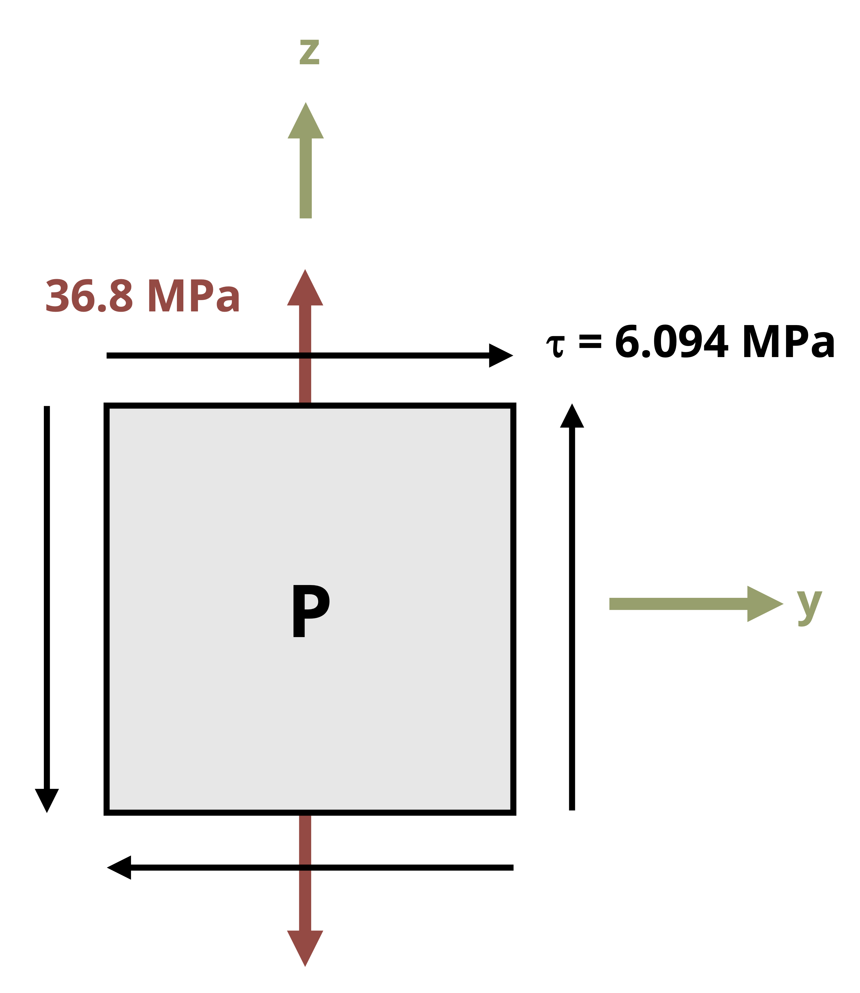
Now find the principal stresses and max/min shear stress. Start by representing the general stress state on a stress element.

We can use the simplified version of the principal stress and the max/min shear equation (Equation 12.5); however, these equations were generally written for stresses in the x-y plane.

\[ \begin{aligned} & \sigma_{1,2}=\frac{\sigma_x+\sigma_y}{2} \pm \sqrt{\left(\frac{\sigma_x-\sigma_y}{2}\right)^2+\tau_{x y}{ }^2} \\[10pt] & \tau_{\max , \min }= \pm \sqrt{\left(\frac{\sigma_x-\sigma_y}{2}\right)^2+\tau_{x y}{ }^2} \end{aligned} \]

In this problem point P is on the y-z plane. Based on the discussion at the end of Section 12.2.2., we can replace the x subscripts with y and the y subscripts with z. Thus the equations become

\[ \begin{aligned} \sigma_{1,2}&=\frac{\sigma_y+\sigma_z}{2}\pm\sqrt{\left(\frac{\sigma_y-\sigma_z}{2}\right)^2+\tau_{yz}^2}\\[10pt] &=\frac{0+36.77{~MPa}}{2} \pm \sqrt{\left(\frac{0-36.77{~MPa}}{2}\right)^2+(6.094{~MPa})^2}\\[10pt] &=37.75{~MPa}, -0.984{~MPa} \\ \end{aligned} \]

\[ \begin{aligned} \tau &=\pm\sqrt{\left(\frac{\sigma_y-\sigma_z}{2}\right)^2+\tau_{yz}^2}\\[10pt] &=\pm\sqrt{\left(\frac{0-36.77 MPa}{2}\right)^2+(6.094 MPa)^2}\\[10pt] &=\pm 19.37 MPa \end{aligned} \]

Answer:

σ₁ = 37.75 MPa

σ₂ = -0.984 MPa

τ_min = -19.37 MPa

τ_max = 19.37 MPa

Summary

Click to expand

NoteKey Takeaways

The overall general stress state for any given point on a loaded body is found by calculating and combining all forms of normal stress and all forms of shear stress.

The combined normal stress at a point comes from normal forces, bending stress, and pressure.

• Normal forces are those perpendicular to the cross-section where the point in question is located. These are also the forces in the longitudinal direction.

  • Normal forces that pull on the body are tensile (positive).

  • Normal forces that push on the body are compressive (negative).

• The bending moment contribution to normal stress comes from bending moments around the centroidal cross-sectional axes.

  • In bending, visualizing the bending shape of a body can determine if a point will be in tension or compression. A point that is located on the outside part of the bend will be in tension and a point on the inside part of the bend will be in compression.

  • Alternatively, use the visual aid described in Section 14.1 to help determine if the bending results in tension or compression.

• Both normal forces and bending moments will result in normal stress in the longitudinal direction with respect to the location of the cross-section.

Pressure will result in normal stress in two directions (hoop and longitudinal/axial).

• The longitudinal stress will combine with the normal stress from normal forces and bending moments to result in an overall longitudinal stress.

• The hoop stress will be the only normal stress in the cross-sectional directions for the situations considered in this text.

• Stress from internal pressure will always be tensile.

The combined shear stress at a point comes from torsion and transverse shear forces.

• The torsional moment is the moment about the longitudinal axis.

• The transverse shear forces lead in the directions of the cross-sectional axes.

• The signs for shear stress are determined by drawing the stress element and considering the direction of the internal torque or shear force on the element’s cut edge relative to the positive and negative faces.

NoteKey Equations

\[ \sigma_L= \pm\left|\frac{F_L}{A}\right| \pm\left|\frac{M_V d_H}{I_V}\right| \pm\left|\frac{M_H d_V}{I_H}\right|+\frac{p r}{2 t} \]

\[ \sigma_{hoop}=\sigma_V=\sigma_H=\frac{p r}{t} \]

\[ \tau= \pm\left|\frac{T c}{J}\right| \pm\left|\frac{V_H Q_V}{I_V t_V}\right| \pm\left|\frac{V_V Q_H}{I_H t_H}\right| \]

where

L = Longitudinal axis

V = Vertical centroidal axis of the cross-section

H = Horizontal centroidal axis of the cross-section

𝜎 = Normal stress [Pa, psi]

A = Cross-sectional area [m², in.²]

F_L = Internal normal force in the longitudinal direction [N, lb]

A = Cross-sectional area [m², in.²]

M_V = Bending moment around the vertical axis of the cross-section [N⸱m, lb⸱in.]

M_H = Bending moment around the horizontal axis of the cross-section [N⸱m, lb⸱in.]

d_H = Horizontal distance between the point on the cross-section for which the stress is being calculated and the V-axis [m, in.]

d_V = Vertical distance between the point on the cross-section for which the stress is being calculated and the H-axis [m, in.]

I_V = The second moment of area about the vertical axis of the cross-section [m⁴, in.⁴]

I_H = The second moment of are about the horizontal axis of the cross-section [m⁴, in.⁴]

p = Internal pressure [Pa, psi]

r = Inner radius of pressure vessel [m, in.]

t (for the pressure term) = Wall thickness of pressure vessel [m, in.]

𝜏 = Shear stress at point of interest [Pa, psi]

T = Internal torque [N·m, lb·in.]

𝜌 = Radial distance from centroid to point of interest [m, in.]

J = Polar moment of inertia [m⁴, in.⁴]

V_H = Internal horizontal shear force [N, lb]

V_V = Internal vertical shear force [N, lb]

Q_V = First moment of area about the vertical axis passing through the point of interest [m³, in.³]

Q_H = First moment of area about the horizontal axis passing through the point of interest [m³, in.³]

t_V = Vertical thickness of the cross-section [m, in.]

t_H = Horizontal thickness of the cross-section [m, in.]

References

Click to expand

Figures

All figures in this chapter were created by Kindred Grey in 2025 and released under a CC BY license.